Jacobi vs. Gauss Seidel - Notes for Dummies

Summary:

Intro
The Coding Explanation
- What's the Difference?
- Which is Better?
The Mathy Explanation

Intro

In numerical analysis, Jacobi Iteration and the Gauss Seidel method are classic examples of iterative methods. However, since most classes focus mainly on deriving the equations, it is easy for the underlying intuition to be buried under a mountain of mathematical symbols and pseudocode. After reading the explanations online, I felt like I understood each step of the derivation, but confused about the more practical side of things: How are these two algorithms different? What are the pros and cons of each? This post contains some of my notes.

Also, shoutout to Dillon Grannis for clarifying a lot of the mathematical concepts!

That's enough context. Let's get started.

The Coding Explanation

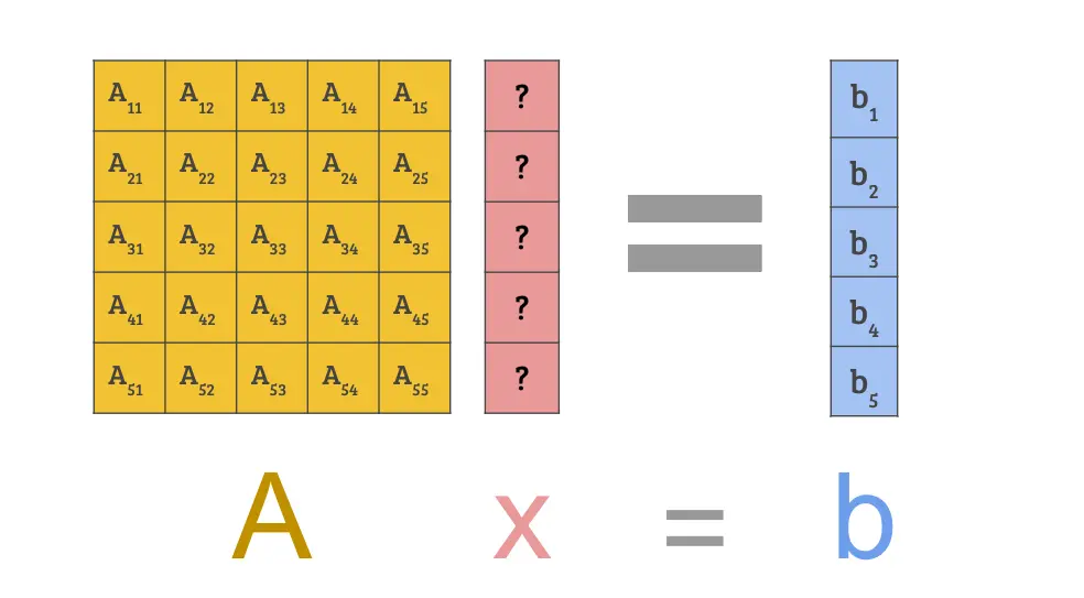
Essentially, we have a system $Ax=b$ , where $A$ is a matrix and $x,b$ are vectors. We know values of matrix $A$ and vector $b$ but not vector $x$ :

Under this condidion, here is a crash course on the two methods:

If $A$ follows certain conditions, the Jacobi Iteration can find a better approximation of $x$ given $A$ , $b$ , and a current approximation $x'$ .
If $A$ follows slightly more conditions, the Gauss Seidel method can do the same as Jacobi, but with better performance.
Practically, we start from some approximation and run one of the two methods many times until we are satisfied with the result.
Usually, we denote the $k^{th}$ guess $x^{(k)}$ to keep track of the iterations. In this language, each mathod takes in $A$ , $b$ , $x^{(k-1)}$ and produces $x^{(k)}$ as a better guess.

What's the Difference?

Both methods provide a formula to compute the $i^{th}$ term of $x^{(k)}$ , which we call $x^{(k)}_i$ , using the subscript to indicate the elements within the vector.

In the two methods, the formula (denoted "f" in the image) is actually the exact same, the only difference being the order we update the values.

In Jacobi Iteration we compute the entire $x^{(k)}$ from $x^{(k-1)}$ :

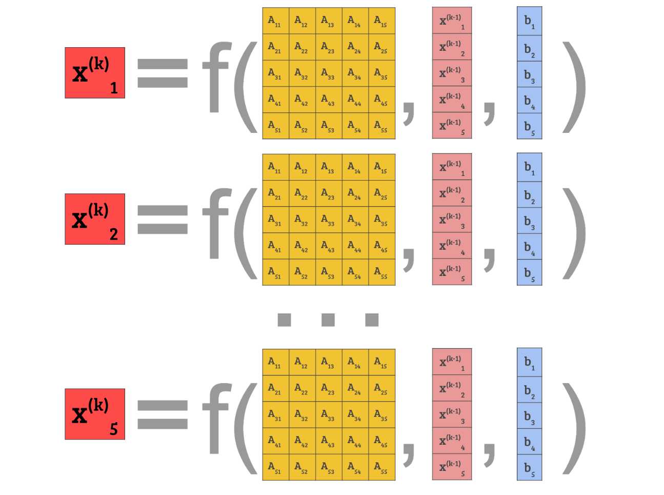
Then we throw away the $x^{(k-1)}$ vector as a whole, replacing it with the new guess $x^{(k)}$ .

In Gauss Seidel method, however, we throw away $x^{(k-1)}_i$ right after computing $x^{(k)}_i$ .

After finishing the computation, we just need to replace the last term before starting the new iteration.

Which is Better?

Pros of Jacobi Over Gauss Siedel:

Jacobi has less strict requirements than Gauss Seidel, so certain classes of questions can only be computed with Jacobi iteration.
Jacobi is very good for distributed programming, since $x^{(k)}_i$ for different values of $i$ can be computed simutaneously on different computers.

Pros of Gauss Siedel Over Jacobi:

Gauss Siedel generally has better performance over Jacobi, since it uses updated values immediately and don't have to wait for the entire vector to finish.
Gauss Siedel can save a lot of space, since we don't need to keep track of both $x^{(k)}$ and $x^{(k-1)}$ at the same time. Gauss Siedel only need one vector of memory, while Jacobi needs two.

The Mathy Explanation

To begin with, this is NOT a rigorous proof! We will be making many assumptions throughout this section without diving into the details, and a math textbook would be a much better source of information if you are looking for Lemmas and Theorems.

Instead, this section contains a quick rundown of the intuiton behind these algorithms, with some equations sprinkled throughout.

Linear Algebra 101: How to Approximate

Let's start simple. Given any invertible matrix $M$ :

MM^{-1} = I

Similarly. Given any invertible matrix $(I-M)$ :

(I-M)(I-M)^{-1} = I

That's a good warmup. Now we can look at something more interesting. Let's replace $(I-M)^{-1}$ with a sum of powers of $M$ and see what we get:

\begin{aligned} &\hspace{0.2in} (I-M)(M^0 + M^1 + M^2)\\ &= (I-M)(I + M + M^2)\\ &= (I-M)I + (I-M)M + (I-M)M^2\\ &= (I-M) + (M-M^2) + (M^2-M^3)\\ &= I-M^3 \end{aligned}

Note how the terms cancel out with each other! The same rule holds if we add more powers of $M$ . Since all consecutive terms cancel out except for the first and the last, we have:

(I-M) (M^0 + M^1 + M^2 + ... + M^k) = I-M^{k+1}

Or, if we want to write it formally and save some space:

(I-M) \sum_{i=0}^k M^i = I-M^{k+1}

We now make an assumption about $M$ : Suppose $M^k$ becomes smaller and smaller as its power goes up. In other words, $M^k$ gets smaller as $k$ gets bigger. $M^{k}$ gets super close to zero as $k$ gets super large.

More formally in terms of limit, we can write it as:

\lim_{k\to\infty}M^{k} = 0

We can make a very similar claim regarding $M^{k+1}$ :

\lim_{k\to\infty}M^{k+1} = 0

Now we can plug this limit into the above equation, where the right hand side is $I-M^{k+1}$ , which gets super close to just $I$ as $k$ gets super large.

More formally in terms of limit, we can write it as:

\lim_{k\to\infty} (I-M) \sum_{i=0}^k M^i = \lim_{k\to\infty} I + M^{k+1} = I

Recall that we have seen another equation with $I$ on the right hand side:

(I-M)(I-M)^{-1} = I

Putting the pieces together, we have:

(I-M)(I-M)^{-1} = \lim_{k\to\infty} (I-M) \sum_{i=0}^k M^i

(I-M)(I-M)^{-1} = (I-M) \lim_{k\to\infty} \sum_{i=0}^k M^i

(I-M)^{-1} = \lim_{k\to\infty} \sum_{i=0}^k M^i

And, if $k$ is large enough:

(I-M)^{-1} \approx \sum_{i=0}^k M^i

As long as $M$ is a nice matrix, in the sense that $(I-M)^{-1}$ exists and $M^k$ gets smaller as $k$ gets bigger, we can use the above logic to approximate $(I-M)^{-1}$ with sums of $M^i$ .

Approximate, but in Linear Systems

Now that we know how to approximate things, we can try to apply what we've learned to a linear system. Consider the following (familiar) scenario, where we know values of matrix $A$ and vector $b$ but not vector $x$ :

Ax = b

Let's try to reframe it into something more familiar.

Define a matrix $M = I-A$ so we have $A = I-M$ :

(I-M)x = b \implies x = (I-M)^{-1}b \approx (\sum_{i=0}^k M^i)b

That looks familiar! Rewrite the above equation into a easy to read format, we essentially have:

x \approx (M^0 + M^1 + M^2 + M^3 + M^4 + ...)b

The more terms of $M^i$ we have, the more accurate the result would be!

One step further: Jacobi and Gauss Seidel

Finally, we can get to the meat: What is exactly going on in Jacobi and Gauss Seidel?

They essentially does what we did above, but took it one step further by breaking the matrix $A$ into two parts:

A = G + B

$G$ is the "good" matrix and $B$ is the "bad" matrix. Both matrices are of the same size, but there is a key difference: Only the good matrix is guaranteed to be easily invertible. The bad matrix can be either hard or impossible to invert.

As a result, we are okay with computing $G^{-1}$ but not $B^{-1}$ .

After we break $A$ down, let's look at the linear system again:

(G + B)x = b

Since we are okay with calculating $G^{-1}$ , we can multiply both sides with it:

\begin{aligned} G^{-1}(G + B)x &= G^{-1}b\\ (G^{-1}G + G^{-1}B)x &= G^{-1}b\\ (I + G^{-1}B)x &= G^{-1}b \end{aligned}

This is looking a bit more familiar, but not quite enough.

Let's rewrite it some more. Define $M = -G^{-1}B$ and $b' = G^{-1}b$ , we plug them into the equation:

\begin{aligned} (I - M) x &= b'\\ x &= (I - M)^{-1} b' \end{aligned}

Applying the formula from the last section:

x \approx (M^0 + M^1 + M^2 + ...)b'

Voila! We have our approximation. Or, expanding the formula into $G$ and $B$ :

x \approx \Big( (-G^{-1}B)^0 + (-G^{-1}B)^1 + (-G^{-1}B)^2 + ... \Big) G^{-1}b

Essentially, this is what Jacobi and Gauss Seidel are doing, although they broke $A$ down differently:

Jacobi chose $G$ to be just the diagonal, and $B$ is everything but the diagonal.
Gauss Seidel chose $G$ to be both the diagonal and everything below the diagonal, and $B$ is everything above the diagonal.

Tying the Math to the Code

The above explanation still begs a question: How do we compute that, exactly?

Both Jacobi and Gauss Seidel are iterative methods, so they perform the computation in iterations. Every new iteration makes an improvement on top of the previous one and produces a more reliable result.

The intuition is for us to add one term of $M^i$ in every iteration:

x^{(k-1)} = (M^0 + M^1 + ... + M^{k-1})b

x^{(k)} = (M^0 + M^1 + ... + M^k)b

However, we don't want to recompute everything on each step since that takes up a lot of space in the computer. How can we compute the iteration while minimizing the cost?

Ideally, we can just use the values of $M$ , $b$ , and $x^{(k-1)}$ to perform the computation. The key is in the following equation:

\begin{aligned} Mx^{(k-1)} &= M(M^0 + M^1 + ... + M^{k-1})b\\ &= (M^1 + M^2 + ... + M^k)b\\ &= (M^0 + M^1 + M^2 + ... + M^k)b - M^0b\\ &= x^{(k)} - M^0b\\ &= x^{(k)} - b\\ \end{aligned}

After shuffling the terms, we have:

\begin{aligned} x^{(k)} &= Mx^{(k-1)} + b\\ \end{aligned}

And that is it! Of course, when we are applying Jacobi or Gauss Seidel, we are operating with the good and the bad matrix under the hood:

\begin{aligned} x^{(k)} &= (-G^{-1}B)x^{(k-1)} + G^{-1}b\\ \end{aligned}

This can also be written as:

\begin{aligned} x^{(k)} &= G^{-1}b - (G^{-1}B)x^{(k-1)}\\ \end{aligned}

This would be the general form we need to perform the computation.

The exact formula of Jacobi and Gauss Seidel are then derived from writing each term down and expanding them, which is some painstacking calculation that I am not going to type up in latex. If you trust me, here are the formulas for solving $Ax=b$ .

Jacobi:

x_i^{(k)}=\frac{1}{a_{i i}}\left[\sum_{\substack{j=1, j \neq i}}^n\left(-a_{i j} x_j^{(k-1)}\right)+b_i\right]

Gauss Seidel:

x_i^{(k)}=\frac{1}{a_{i i}}\left[-\sum_{j=1}^{i-1}\left(a_{i j} x_j^{(k)}\right)-\sum_{j=i+1}^n\left(a_{i j} x_j^{(k-1)}\right)+b_i\right]

In Gauss Seidel, we skipped quite a bit of computation by using the already computed terms in $x^{(k)}$ instead of revisiting all the terms in $A$ .

In coding practice, the similarity in formulas makes Gauss Seidel almost the same as Jacobi, the only difference being we are throwing away $x^{(k-1)}_i$ immediately after $x^{(k)}_i$ is computed in Gauss Seidel, while in Jacobi we wait until the entire vector $x^{(k)}$ is computed before throwing away $x^{(k-1)}$ all together.